The pizza delivery process

In this section, we’ll illustrate the process of simulating a business scenario using our Pizza Delivery template. This example mirrors a real-world situation from two perspectives: the customer and the pizza vendor.

Pizza delivery process open in the Simulation environment

The pizza vendor is aware of a problem: delivery times are too long, and customers are increasingly complaining. The goal of the initial simulation is to gather real data based on the current resources in use, so the vendor can identify issues and improve the delivery process. Subsequent simulations will test potential solutions to this problem, allowing the vendor to refine the process and optimize delivery times.

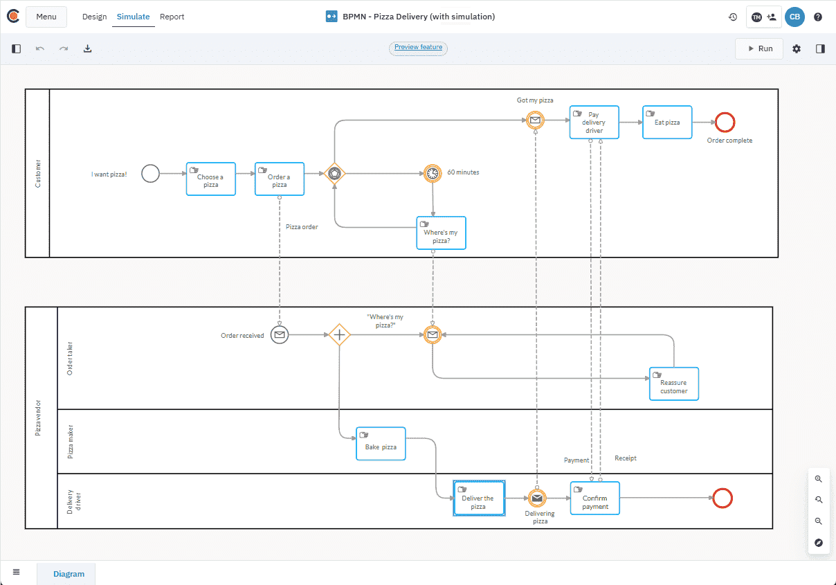
The process is straightforward: a customer places an order with the pizzeria. The person taking the order passes the order to the pizza maker, who prepares the pizza, which is then handed off to a delivery driver. The delivery driver takes the pizza to the customer. The process also accounts for the situation where the pizza isn’t delivered within the promised time.

For the pizza vendor, the primary objectives are to fulfill the order efficiently, ensure timely delivery and keep costs and resources to a minimum in order to make a profit. The vendor aims to speed up the order-to-delivery time, optimize resource usage (the number of staff and the delivery method, such as bike versus motorcycle), and keep operational costs low.

The resources available to the vendor are as follows:

Order taker
Pizza maker
Delivery driver

To represent the different perspectives of the customer and vendor, the simulation diagram uses two pools: one for the customer and one for the vendor.

Customer: The customer places an order with customer service and then waits for delivery. If delivery isn’t completed within the expected time, the customer calls to inquire about the status of the delivery. The order taker then checks with the delivery driver and pizza maker to ascertain the status of the order.

Pizza vendor: The pizza vendor’s process includes order reception, order preparation by the pizza maker, delivery handoff, payment collection, and order closure. The vendor side of the process also addresses the scenario where the order taker receives a complaint, causing the process to diverge and requiring the order taker to resolve the issue by speaking to the pizza maker and deliver driver to identify the cause of the problem, rectify the issue and ensure the customer is satisfied.

Additionally, the simulation considers two distinct calendars — one for weekdays and another for weekends — reflecting the increase in customer orders during the weekend, which impacts the pizza vendor’s resource requirements.

Process parameters

Parameter values are fundamental in shaping the behavior and interactions of elements within a business process simulation and for generating accurate and reliable simulation results. They define how tasks, resources, gateways, and events operate and interact with one another. By adjusting parameter values, such as processing times, costs and resource requirements, you can replicate the real-world variables that influence how the process flows. The ability to customize these values ensures that the simulation reflects current operational conditions, providing a baseline from which adjustments can be made as results come in.

In the context the pizza delivery process, parameter values help us simulate key aspects of the process such as order frequency, delivery times, and resource costs and availability. Setting these parameters to reflect the current situation enables us to evaluate how the process performs under typical conditions. Once the simulation results are gathered, we can adjust these values to fine-tune the process and explore how different parameters impact efficiency. This iterative approach ensures that the final model reflects realistic scenarios and provides actionable insights.

For the pizza delivery model, we’ll be focusing on these parameters.

Trigger time parameters

Start events mark the beginning of a process. When modeling for simulation, setting the right trigger time parameters is essential to accurately reflect how the process begins. These parameters control triggers, timing, and data flow.

Trigger count

Trigger count defines the maximum number of times the start event will trigger within a specified period. This parameter helps simulate how many times the process is initiated, allowing you to model scenarios where the process is triggered multiple times in a given frame of time. By adjusting the trigger count, you can explore how varying demand or event occurrences impact the process flow.

Inter trigger timer

Inter trigger timer defines the time interval between consecutive occurrences of the start event. This parameter is useful for simulating processes that are triggered at regular intervals or triggered at the intervals determined by a distribution. By adjusting the inter trigger timer, you can model scenarios where the process needs to handle different timing patterns.

Time parameters

Time parameters define how each step in the process is performed during a simulation, affecting the duration and resource usage of each task.

Processing time

Processing time simulates how long each task takes to complete. It can be set using a fixed value or a more detailed time format, or using distributions to account for variability and randomness in task durations.

Cost parameters

Costs represent the financial impact associated with completing each task. These costs can be set as fixed amounts, which remain constant regardless of the task’s duration, or as unit costs, which reflect ongoing expenses that fluctuate depending on the processing time. Defining both fixed and variable costs enables you to simulate the financial dynamics of the process and evaluate how different scenarios affect overall profitability.

Task costs

Task costs represent the financial expenditure associated with completing each task in the process. These costs can be set as fixed or unit costs. Defining task costs is essential for evaluating how each task impacts overall expenses, allowing for more precise budgeting, cost control, and profitability analysis.

Resource costs

Resource costs represent the financial expenses associated with using each resource. These costs can be set as fixed or unit costs. Defining resource costs helps identify the financial impact of resource usage and provides insights into how changes in resource costs may affect overall process profitability.

Resource Parameters

Resource parameters define the resources required to support the tasks in the process, including both the quantity and associated costs.

Resource requirements

Task resource requirements specify the resources needed to complete each task. These can include personnel, equipment, or materials. Resource requirements can be set based on the type and quantity of resources needed, allowing us to model how resource availability or constraints impact the task’s execution. By adjusting these parameters, you can simulate different resource allocation strategies and identify the optimal setup for efficient task completion. This helps pinpoint resource bottlenecks and optimize resource utilization across the process.

Resource quantity

Resource quantity refers to how many resources are needed to complete the tasks in the process. This can include the number of employees, pieces of equipment, or units of material required at each step. By adjusting resource quantities, we can simulate different resource allocation scenarios and assess the impact of resource availability on process efficiency.

Parameter formats

For some parameters it’s important to consider the format in which they’re expressed. This ensures accuracy and allows for the flexibility needed to simulate various real-world conditions. Parameters can be set using either fixed values or distributions to account for variability in the process.

Fixed Values

Fixed values are used for determining constants like time intervals. They can be expressed in two formats:

Short format: This format uses a single value to define the time interval between triggers, such as seconds, minutes, hours, days, weeks, months, or years. For example, you might set a trigger to occur every 5 days.

Long format: In contrast, the long format provides a more detailed definition of the time interval, using multiple values. For instance, you can define a trigger to occur every 3 days, 2 hours, and 1 minute. This provides more granular control over the timing.

Distributions

In many scenarios, processes are subject to variability. To simulate this, distributions can be applied to parameters, allowing you to model a range of values instead of a fixed point. The following distribution types offer different ways to incorporate randomness into your simulation:

Distribution	Description
Beta	A continuous probability distribution defined by two positive parameters. It’s often used to model random variables that are constrained within a range, such as percentages or probabilities.
Binomial	Models the number of successes in a fixed number of independent trials, each with the same probability of success. It is commonly used for scenarios with two possible outcomes, such as yes/no or success/failure.
Gamma	A continuous probability distribution defined by two positive parameters: shape and rate, and is useful for modeling processes that involve a series of events.
Log normal	A continuous probability distribution of a variable whose logarithm is normally distributed. It’s often used to model variables that are positively skewed, such as stock prices or income.
Poisson	Used to model the number of unpredictable events within a unit of time. It’s often used to model rare or random events.
Triangular	A continuous probability distribution shaped like a triangle, defined by a minimum, maximum, and mode. It’s often used when only limited information is available about the range and likely outcome of a process.
Truncated normal	A variation of the normal distribution that is restricted within a specific range. It’s useful for modeling processes where values outside a certain interval are not possible or realistic.
Uniform	A continuous probability distribution where all outcomes are equally likely within a specified range. It’s often used in simulations to model situations with no bias toward any specific outcome.
Weibull	A continuous probability distribution commonly used to model life data, reliability, and failure times. It’s defined by a shape parameter and a scale parameter, and it can model both increasing and decreasing failure rates.
Custom	Allows you to define a specific set of probabilities or values based on your data or specific needs. It provides flexibility to model scenarios where standard distributions don’t apply or aren’t sufficient.

Follow along with the template

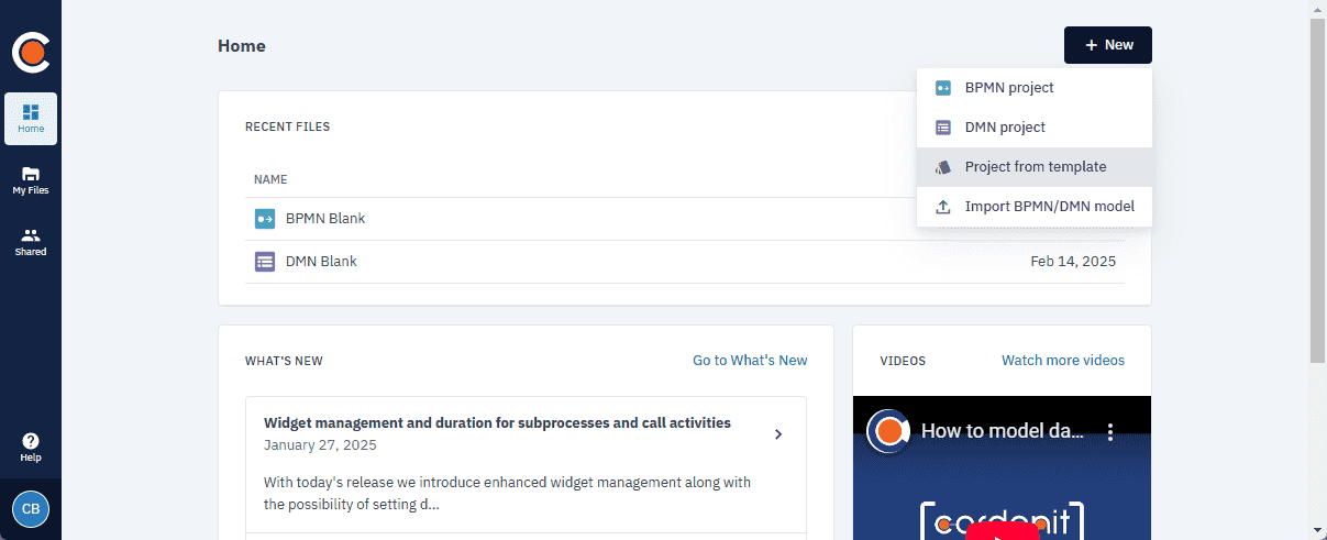
To follow along, you can create a project using the provided template, which will allow you to replicate the steps outlined here.

From the Cardanit Home page or My Files, in the header, click New.
Select Project from template.
In the page that opens, select BPMN - Pizza Delivery (with simulation).